
Getting the statistical signficance from the acf function.
The R language provides us with a useful method to calculate the autocorrelation function (ACF) of a time series. An example of an environmental time series with a seasonal cycle is shown below, with the resulting plot:
corr <- acf(series, lag.max=288,type="correlation",plot=TRUE,na.action=na.pass)
(My data set has some missing values, hence the na.action=na.pass parameter.)
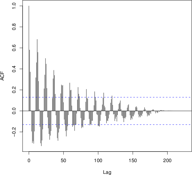
As well as the calculated ACF, we can see two blue dashed lines across the plot. These lines indicate the point of statistical significance - values between these lines and zero are not statistically significant, while those above and below the lines (towards one and minus one) are significant.
In some cases, it would be useful to know what this value is, so we can determine whether individual values from the ACF are significant or not. Unfortunately the output of R’s acf function doesn’t make it available to us.
A hunt through the source code of the acf function gives us the information we need. We can calculate the significance level as follows:
corr <- acf(series, lag.max=288,type="correlation",plot=TRUE,na.action=na.pass)
significance_level <- qnorm((1 + 0.95)/2)/sqrt(sum(!is.na(series)))
The 0.95 parameter indicates that we calculate the correlation at which values
are significant to the 95% level - you can change this as you see fit.
Note that the significance is a function of the number of data points you have -
the more points, the closer to zero the significance level will be, and the more
confidence you can have in your ACF.